


Drag is a force exerted on an object moving through a fluid, and it is oriented in the direction of relative fluid flow. Drag acts opposite to the direction of motion and tends to slow an object. As an example, think of running against a high wind and feeling the drag pushing you back in the direction of relative fluid flow. This same force acts on spacecraft and objects flying in the space environment. Drag has a significant impact on spacecraft in low Earth orbit (LEO), generally defined as an orbit below an altitude of approximately 2,000 kilometers (1,200 mi). Although the air density is much lower than near the Earth’s surface, the air resistance in those layers of the atmosphere where satellites in LEO travel is still strong enough to produce drag and pull them closer to the Earth (Figure 1, shown above, the region of the Earth’s atmosphere where atmospheric drag is an important factor perturbing spacecraft orbits.(NASA/GSFC)). The International Space Station (ISS) and the Hubble Space Telescope are examples of spacecraft operating in LEO.
The drag force on satellites increases during times when the Sun is active. When the Sun adds extra energy the atmosphere the low density layers of air at LEO altitudes rise and are replaced by higher density layers that were previously at lower altitudes. As a result, the spacecraft now flies through the higher density layer and experiences a stronger drag force. When the Sun is quiet, satellites in LEO have to boost their orbits about four times per year to make up for atmospheric drag. When solar activity is at its greatest over the 11-year solar cycle, satellites may have to be maneuvered every 2-3 weeks to maintain their orbit [1].
In addition to these long-term changes in upper atmospheric temperature and density caused by the solar cycle, interactions between the solar wind and the Earth’s magnetic field during geomagnetic storms can produce large short-term increases in upper atmosphere temperature and density, increasing drag on satellites and changing their orbits. The North American Aerospace Defense Command (NORAD) has to re-identify hundreds of objects and record their new orbits after a large solar storm event (Figure 2). During the March 1989 storm event, for example, the NASA's Solar Maximum Mission (SMM) spacecraft was reported to have "dropped as if it hit a brick wall" due to the increased atmospheric drag.
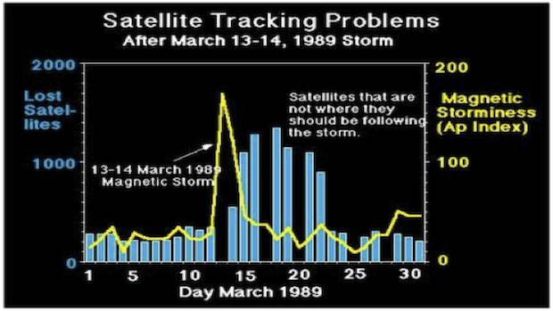
Figure 2. Number of satellites lost in connection with the March 13-14, 1989 storm (UCAR).
The impact of satellite drag and the current efforts to model it are discussed in the following excerpt from Fedrizzi et al., 2012 [2]:
It is extremely important to keep track of spacecraft and objects flying in the space to avoid collisions with space junk and orbital debris that may be in their path. Collision avoidance has become of increasing concern due to the recent accidental hypervelocity collision of two intact spacecraft in February, 2009. The collision occurred at an altitude of 790 km, leaving pieces of debris that have been gradually separated into different orbital planes around the Earth, threatening other satellites for the next few decades. Since 1957, more than 25,000 artificial space debris have been cataloged (Figure 3), many of which have naturally decayed into the lower atmosphere. Currently, the U.S. Space Surveillance Network (SSN) tracks over 20,000 man-made objects larger than 10 cm in size, which are known as the “catalogued” population. Debris between 1 cm and 10 cm (approximately 500,000), referred to as the “lethal” population, are the most concerning as they cannot be tracked or cataloged and can cause catastrophic damage when colliding with a satellite. Objects smaller than 1 cm (approximately 135 million measuring from 1mm to 1cm, and many more smaller than 1 mm) that could disable a satellite upon impact are termed the “risk” population [3].
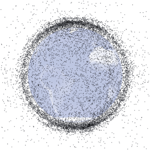
Figure 3. Thousands of manmade objects—95 % of them “space junk”— occupy low Earth orbit. Each black dot in this image shows either a functioning satellite, an inactive satellite, or a piece of debris. Although the space near Earth looks crowded, each dot is much larger than the satellite or debris it represents, and collisions are extremely rare. (NASA illustration courtesy Orbital Debris Program Office.)
The consequences of a spacecraft collision with debris can range from performance degradation to failure and satellite fragmentation. In LEO, debris as small as a few millimeters in diameter can puncture unprotected fuel lines and damage sensitive components, while debris smaller than 1 mm in diameter can erode thermal surfaces and damage optics. Although smaller objects can partly be mitigated through the use of meteor bumpers, such as on the ISS, the only way to mitigate larger objects impact is to maneuver the spacecraft to avoid collision. Such maneuvers are expensive, impact the operation of sensitive experiments on board, and ideally should only be done if the chance of collision is high. To assess the risk, and mitigate the likelihood of collision, the SSN monitors these objects and predicts their orbits about three days ahead.
Orbit propagation models are used to determine the location of space objects in the relatively near-term (typically over a period of a few days or less) for purposes of collision avoidance or re-entry predictions, and also to make long-term predictions (typically over a period of years) about the debris environment. Both short- and long-term propagation models must take into account the various forces acting on space objects in Earth’s orbit including atmospheric drag. Since accurate orbit propagation models that include all forces acting on an orbiting object can be very computation intensive, most models take into account only the forces that most strongly affect the space objects in particular orbital regions. The primary forces acting on a space object in LEO are atmospheric drag and gravitational attraction of the Earth [4].
The largest uncertainty in determining orbits for satellites operating in low Earth orbit is the atmospheric drag. Drag is the most difficult force to model mainly because of the complexity of neutral atmosphere variations driven by the Sun, and the propagation from below of lower atmosphere waves [5, 6]. Atmospheric neutral density models routinely used in orbit determination applications are mainly empirical. These models are based on historical observations to which parametric equations have been fitted, representing the known variations of the upper atmosphere with local time, latitude, season, solar and geomagnetic activity [7, 8, 9]. First-principle (or physics-based) models can also provide information about the atmospheric density conditions. Unlike empirical models, first principles physics models seek to calculate a physical quantity starting directly from established laws of physics without making assumptions such as empirical or fitted parameters. Taking into account the interactions between upper atmosphere winds, composition and densities, first-principle models are able to provide a realistic representation of neutral density in the upper atmosphere if the magnitude, spatial distribution, and temporal evolution of the solar sources can be defined with sufficient accuracy, especially in long-duration magnetic storm events [10].
Going to the CTIPe web page shows a simulation using the coupled thermosphere-ionosphere-plasmasphere electrodynamics (CTIPe; https://www.swpc.noaa.gov/products/ctipe-total-electron-content-forecast) physics-based model [11], illustrates the increase in atmospheric density at 400km altitude during the occurrence of a large magnetic storm on May 15, 2005, as a satellite (represented by the black diamond) flies through. The atmospheric density is given in Kg/m3. As the time progresses, the satellite will encounter denser air following the beginning of the magnetic storm (starting around 06:00 Universal Time). As the storm comes to end, atmospheric density slowly goes back to quiet conditions.
References:
1. “Achieving and Maintaining Orbit”. https://earthobservatory.nasa.gov/features/OrbitsCatalog
2. Fedrizzi, M., T. J. Fuller-Rowell, and M. V. Codrescu (2012), Global Joule heating index derived from thermospheric density physics-based modeling and observations, Space Weather, 10, S03001, doi:10.1029/2011SW000724.
3. Crowther, R. (2003), Orbital debris: A growing threat to space operations, Philos. Trans. R. Soc. London, Ser. A, 361, 157–168, doi:10.1098/rsta.2002.1118.
4. National Research Council (NRC) (1995), Orbital Debris: A Technical Assessment, Natl. Acad. of Sci., Washington, D. C.
5. Marcos, F., B. R. Bowman, and R. E. Sheehan (2006), Accuracy of Earth’s thermospheric neutral density models, paper presented at AIAA 2006–6167, AIAA/AAS Astrodynamics Specialist Conference, Am. Inst. of Aeronatu. and Astronaut., Keystone, Colo., 21–24 Aug.
6. Doornbos, E. (2007), Thermosphere density model calibration, in Space Weather: Research Towards Applications in Europe, Astrophys. Space Sci. Libr. Ser., vol. 344, edited by J. Lilensten, pp. 107–114, Springer, New York.
7. Bruinsma, S., G. Thullier, and F. Barlier (2003), The DTM-2000 empirical thermosphere model with new data assimilation and constraints at lower boundary: Accuracy and properties, J. Atmos. Sol. Terr. Phys., 65, 1053–1070, doi:10.1016/S1364-6826(03)00137-8.
8. Picone, J. M., A. E. Hedin, D. P. Drob, and A. C. Aikin (2002), NRLMSISE-00 empirical model of the atmosphere: Statistical comparisons and scientific issues, J. Geophys. Res., 107(A12), 1468, doi:10.1029/2002JA009430.
9. Bowman, B. R., W. K. Tobiska, F. A. Marcos, C. Y. Huang, C. S. Lin, and W. J. Burke (2008), A new empirical thermospheric density model JB2008 using new solar and geomagnetic indices, paper presented at the AIAA/AAS Astrodynamics Specialist Conference, Am. Inst. of Aeron. and Astron., Honolulu, Hawaii, 18–21 Aug.
10. Fuller-Rowell, T. J., and S. C. Solomon (2010), Flares, coronal mass ejections, and atmospheric responses, in Space Storms and Radiation: Causes and Effects, edited by C. J. Schrijver and G. L. Siscoe, pp. 321–357, Cambridge Univ. Press, New York.
11. Codrescu, M. V., C. Negrea, and M. Fedrizzi, T. J. FullerRowell, A. Dobin, N. Jakowsky, H. Khalsa, T. Matsuo, and N. Maruyama (2012), A real-time run of the coupled thermosphere ionosphere plasmasphere electrodynamics (CTIPe) model, Space Weather, 10, S02001, doi:10.1029/2011SW000736.