

This product enables users to compare Geoelectric fields calculated over the lower 48 states based on the Fernberg (2012) 1D models (used by SWPC's initial operational version) with Geoelectric fields calculated using magnetotelluric survey results. The latter method provides way to model 3D Earth conductivity empirically.
The scatter plots are derived by running the Fernberg 1D model and the empirical 3D model through 93 days of historical geomagnetic observatory data, specifically March 1-31, 1989, July 1-31, 2000, and October 1-31 2003. These are the only three months during cycles 22-24 during which the Kp index reached its maximum of 9o (NOAA scale G5 extreme) for solar cycles 22-24. The inclusion of full months enables the sample to include a full range of geomagnetic activity levels. The input data used 10 USGS observatories and 9 NRCAN (Canadian) observatories with one-minute cadence. These data were detrended and input into a model that uses the method of Spherical Elementary Current Systems (SECS) (Amm & Viljanen 1999 & Pulkkinen et al. 2003) to infer the magnetic field time series on a regular 1/2 degree by 1/2 degree grid over the lower 48 states of the US where the 1D model grid points exist and close to locations where MT surveys are available from the IRIS database.
For the 1D model, a 2 degree x 2 degree geographical grid is defined over the lower 48 states. For each grid point, the physiographic region is determined and one of the 20 Fernberg 1D models is assigned. The magnetic field time series is convolved with the transfer function derived from the 1D model and a geoeletric field time series is thereby derived at the grid point. These are combined over all the grid points resulting in a minute-by-minute series of maps of the geoelectric field for these time periods.
For the 3D empirical model, we take the 1/2 degree by 1/2 degree grid point from the SECS model output nearest to each survey location as the input magnetic field time series. This time series is convolved with the empirical transfer function derived from the survey to generate a geoelectric field time series on an irregular grid. All 1084 survey sites then form an irregular grid of minute-by-minute geoelectric field maps which are then resampled to a regular 1/2 degree by 1/2 degree grid.
For the comparison, we step through each of the 1D grid points on the 2 degree x 2 degree grid. All the 3D empirical outputs that are within a 2 degree square centered on the 1D grid point are averaged together - so effectively the 3D empirical model is smoothed to a 2 degree x 2 degree grid for comparison purposes. We then produce scatter plots for 1D Ex (north) vs 3D smoothed Ex (north), 1D Ey (east) vs 3D smoothed Ex (north), 1D Ey (east) vs 3D smoothed Ex (north), and 1D Ey (east) vs 3D smoothed (north). Each plot includes a count of the number of high resolution (unsmoothed) 3D points that were averaged together.
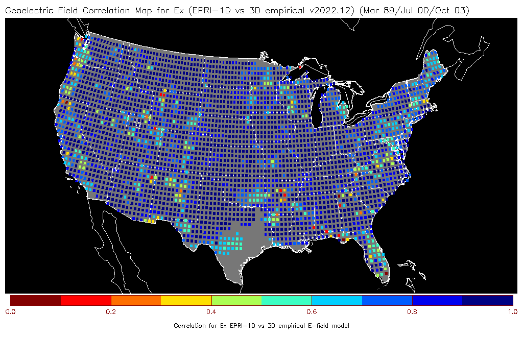
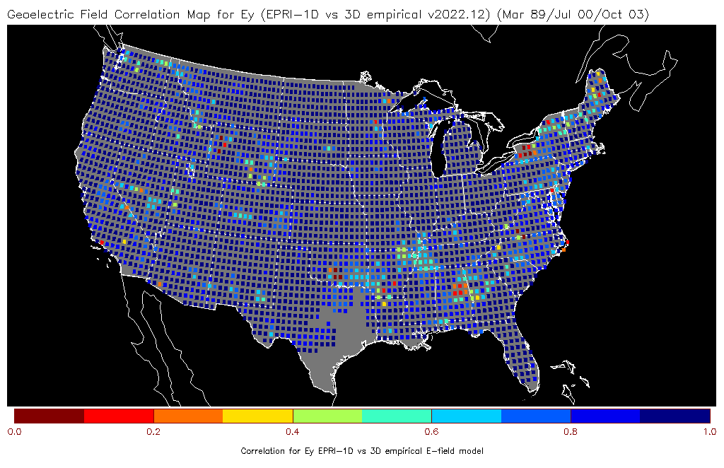
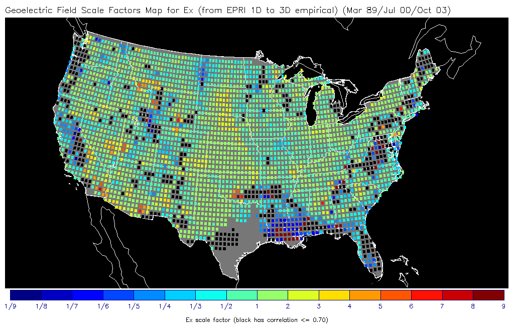
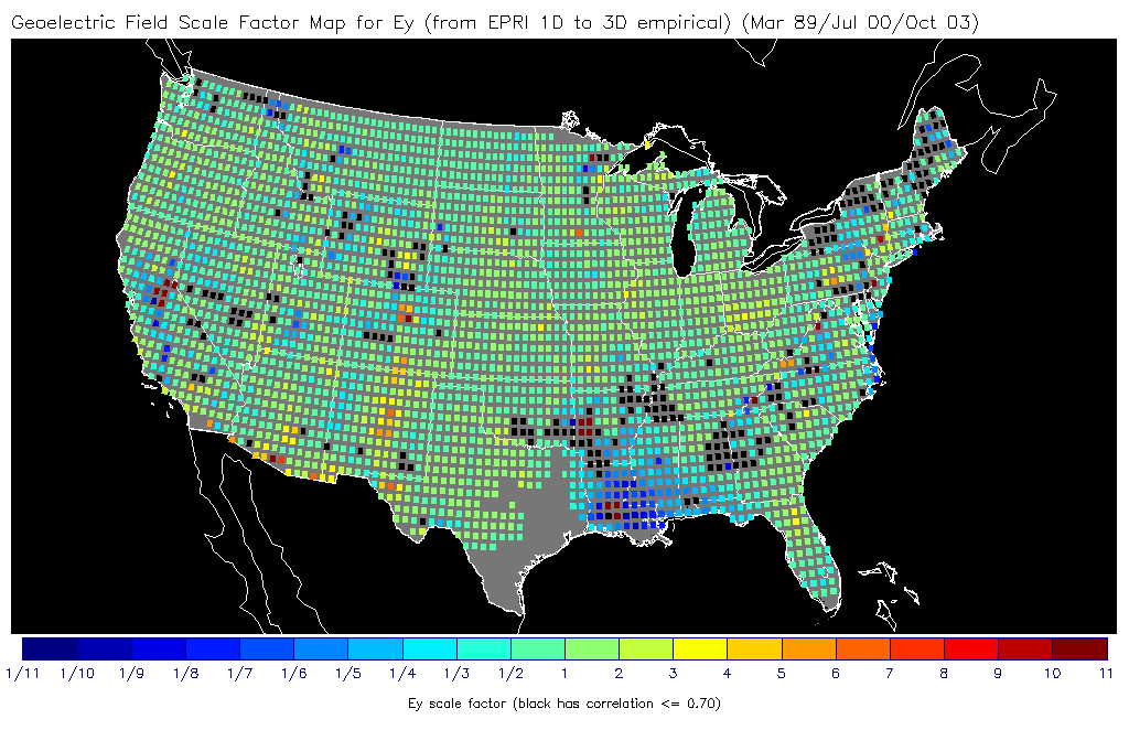
The plots are color coded based the maximum E-field component that was attained so that areas of relative low or high response are quickly identified. A correlation coefficient is included along with a root-mean square (rms) difference of the points and a mean absolute error (mae). For scatter plots with sufficiently high correlation, a slope is also calculated for a linear fit between the points. In locations where the correlations are high, a simple scaling factor could be applied to provide a reasonable mapping between 1D based calculations and 3D smoothed results.
Plots where the northward components (upper left) and eastward components (lower right) are highly correlated while at the same time one sees very little correlation between the cross components (upper right and lower left) are an indication that the survey data are indicating a relatively 1D response, at least at the scale of 2 degree averaging. Areas where this relationship does not hold indicate that the 1D model isn't adequate and the 3D models are a required improvement.
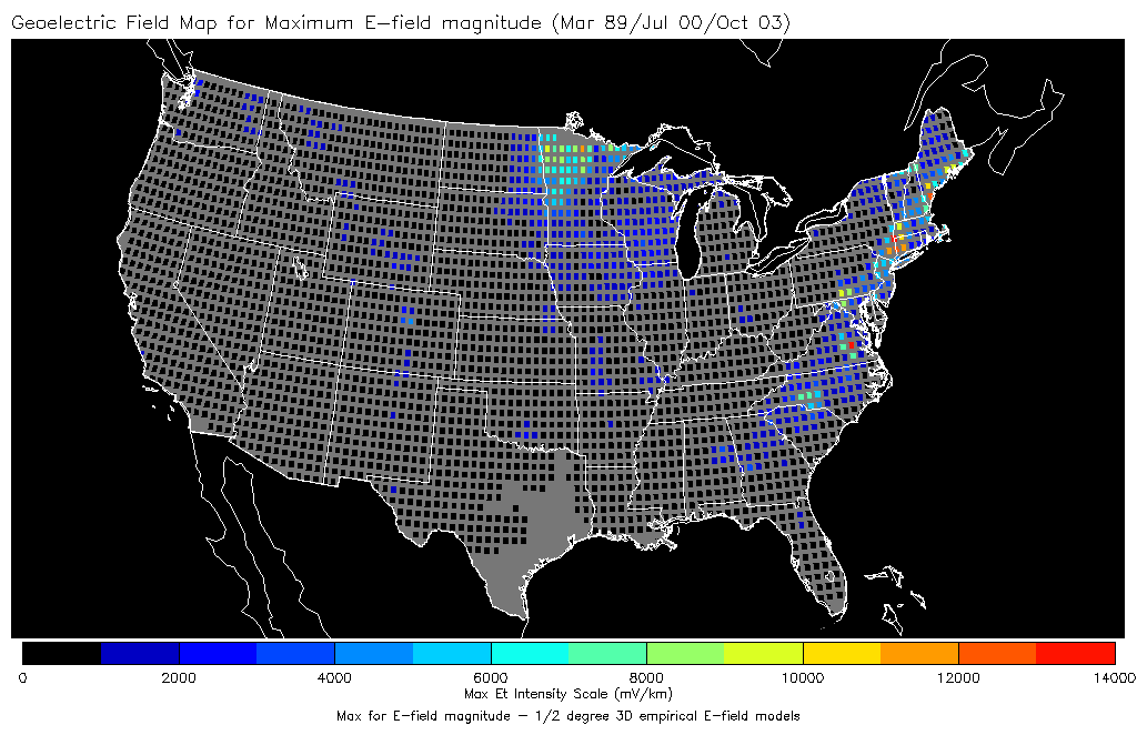
The summary tab provides an overview of the correlations and the scaling factors. The scaling plots enable a quick identification of points where the correlations are poor (the black squares) and also indicate how large the correction factor is between the 1D and the 3D averaged models. The bottom plot on the summary page examines the peak geoelectric field magnitude calculated over these three G5 months on the 1/2 degree resolution grid using the 3D empirical modeling approach.
The impact of geomagnetic storms on the electrical power grid is a potential hazard to the nation’s critical infrastructure. A key requirement identified by the electrical power grid industry to help mitigate this threat is to specify and predict the regional geoelectric field. Once the geoelectric field is known, the level of geomagnetically induced currents in the power grid can be calculated and the potential impact on the power grid can be assessed. In the initial phases of standards development and E-field map product development, much of the work was based on a collection of 1D conductivity profiles as published by Fernberg (2012), and maps based on these models were deployed operationally on NOAA Space Weather Prediction Center’s operational systems in September 2019.
Meanwhile, empirical electromagnetic transfer functions over much of the lower 48 states of the United States have become publicly available through the work of the NSF supported Earthscope US Array project and others and are published as a data product through IRIS (see Kelbert et al, 2011 for more information). The usage of an empirical magneto-telluric transfer function (EMTF) from an MT survey for geoelectric field mapping is expected to provide a more accurate representation of the Earth conductivity then would be possible using a 1D model. In this work we compare time series results for Geoelectric fields using the 1D models for a large number of days, including days with extreme geomagnetic activity, with the results using EMTF’s, to quantify the model differences statistically, thereby providing a guide to the degree one may be able to scale between the two approaches for locations where EMTF’s are available. An update to the geoelectric field map based on EMTF's at 0.5 degree resolution is expected to be deployed operationally at SWPC in September of 2020.
TBD. Please send requests to customer support.